You are heading to a doctor’s appointment and you realize you have to get to the clinic in just ten minutes. When you look at your navigation app, you notice something: a route highlighted in green. Obviously suggesting the fastest way to your destination. This in turn, is a prediction powered by machine learning. Welcome to the future of urban commuting, where traffic prediction with machine learning is revolutionizing the way we travel. By leveraging data and advanced algorithms, it provides real-time insights & forecasts, thereby ensuring that you arrive at your appointment on time and hassle-free.
Traffic prediction plays an essential role in intelligent transportation systems. Notabliy accurate traffic prediction can assist route planning, guide vehicle dispatching, & mitigate traffic congestion. Nevertheless, this problem is challenging due to the complicated and dynamic spatio-temporal dependencies between different regions in the road network. Spatio-temporal dependency refers to the relationship between different regions in the road network that changes over time and space. It describes how traffic conditions in one area can be influenced by conditions in another area, and how these influences evolve over time. As a result, a significant amount of research efforts have been devoted to it, especially deep learning methods, advancing traffic prediction abilities [1].
The research on short-term traffic prediction models has been increased extensively in recent years to improve transport management [2]. An accurate prediction model can play an important role in optimizing freeway operations and avoiding traffic breakdowns. These models have been developed using simulated data or historical field data extracted from detectors attached along the roads. Subsequently, these data become an input to statistical techniques and Artificial Intelligence (AI) based on machine learning models for a short-term traffic predictions [3, 4].
However, the rapid development of big data and complex computational intelligence has created AI models (i.e. deep learning models) that can capture future traffic patterns more accurately than statistical models. An example of recent models are the Uni-directional long short term memory (Uni-LSTM) recurrent neural network and its extension Bidirectional long short term memory (BiLSTM). Previous research has shown that Uni-LSTM models are effective in handling long-term dependencies as they remember useful information from inputs that have already passed through using “additional gates” incorporated in their architectures [5, 6, 7]. If the concepts of Uni-LSTM and BiLSTM seem complex to you. They are simply machine learning models that are highly effective in analyzing and predicting time-dependent data, such as traffic patterns.
Google Maps uses machine learning, including deep learning with Graph Neural Networks, to predict traffic conditions and determine the best routes. The system analyzes historical traffic patterns and combines them with live traffic data to generate accurate predictions. The partnership with DeepMind has improved the accuracy of Estimated Time of Arrival (ETA) predictions. They are now consistently accurate for over 97% of trips. This is made possible using a machine learning architecture known as Graph Neural Networks–with significant improvements in places like Berlin, Jakarta, São Paulo, Sydney, Tokyo, and Washington D.C. This technique is what enables Google Maps to better predict whether or not you’ll be affected by a slowdown that may not have even started yet! [8].
Please note that the aim of this article is to showcase the practical utility of machine learning, rather than to explore its technical complexities. We aim to highlight the applications of machine learning in traffic prediction forecasting with an objective of sparking interest that encourages further exploration into data science and machine learning. If you are looking to learn machine learning, do check our Machine Learning Engineer Track . Start your career as a Machine Learning Specialist!
That being said, let’s take a look at some code snippets to see machine learning in action for traffic prediction using machine learning.
Some of the code snippets in this article are sourced from a Kaggle notebook by Karnika Kapoor, titled “Traffic Prediction: GRU”. Kaggle is a platform that provides a community for data scientists and machine learning practitioners to explore, analyze, and share quality data sets and build machine learning models. It offers a collaborative environment where users can participate in competitions, access a broad range of datasets, and gain insights from other professionals in the field.
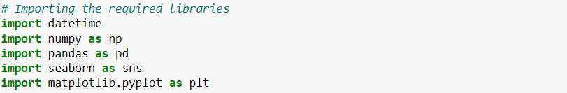
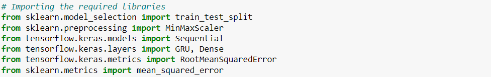
Continuing from our previous discussion on Kaggle, the code snippet below sets up the foundation for a machine learning project focused on traffic prediction. It includes importing essential libraries, such as numpy and pandas for data manipulation, matplotlib and seaborn for data visualization, and datetime for handling date and time data. This setup is crucial for exploring, cleaning, and understanding data before applying any machine learning models. Undoubtedly making it a foundational step in any data science project.
The code below loads datasets from a specified path on Kaggle into a Pandas DataFrame, which is a structure used for data manipulation in Python.


- DATETIME: The date and time of the data entry.
- JUNCTION: Identifier for the traffic junction.
- VEHICLES: The number of vehicles passing through the junction.
- ID: A unique identifier for each data entry.
These features provide information about traffic flow at different junctions over time. It’s worth noting that although the “ID” column was part of the original dataset, it has been removed as it does not contribute to traffic prediction analysis..
Examining summary statistics is beneficial because it provides a quick overview of key characteristics of the numerical data. The code below generates summary statistics for the numerical variables within the dataset and transposes the result to display it in a more readable format.
These statistics include measures like mean (average), standard deviation (a measure of data spread), minimum, maximum, and quartiles. They help data analysts and scientists understand the central tendency, variability, and distribution of the data. This is crucial for making informed decisions about data preprocessing, feature selection, and modeling. Summary statistics also aid in identifying potential outliers or unusual patterns in the data.

- Count: Shows the number of non-missing entries in each column.
- Mean: Provides the average value for each column.
- Std (Standard Deviation): Indicates the amount of variation or dispersion in each column.
- Min: The smallest value in each column.
- 25% (First Quartile): The value below which 25% of the data falls.
- 50% (Median): The middle value of the dataset.
- 75% (Third Quartile): The value below which 75% of the data falls.
- Max: The largest value in each column.
Overview of dataset characteristics with the .describe() method:

Having showcased the value of summary statistics via the .describe() method for understanding the core trends and variations in our data, we now broaden our view by delving into metadata. This approach will further deepen our insight into the data’s framework and attributes (column names or features), enriching our comprehension of the dataset’s intricacies.
Metadata

Metadata provides an overview of the dataset itself; it’s the data about the data. It provides a high-level summary about the characteristics of the dataset. It includes details such as the column names, the types of data contained in each column, and the count of non-null entries in each column, among other aspects. The code snippet below is typically utilized to retrieve the metadata of a dataset.

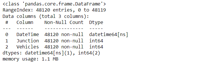
- Range Index: The dataset is indexed from 0 to 48119, providing a unique identifier for each row.
- Columns: There are a total of 3 columns, each representing a different feature or attribute related to traffic flow.
- Column Details: Each column’s non-null count is 48120, indicating no missing values in the dataset.
- Data Types: The dataset consists of datetime (datetime64[ns]) and integer (int64) data types.
- Memory Usage: The dataset consumes approximately 1.1 MB of memory.
One of the primary responsibilities of a data scientist or machine learning practitioner involves communicating findings to stakeholders. Therefore, an integral part of their role is to create visualizations that convey insights derived from data analysis, ensuring that the information is accessible and understandable.
To illustrate this point, let’s take a look into a couple of visualizations:
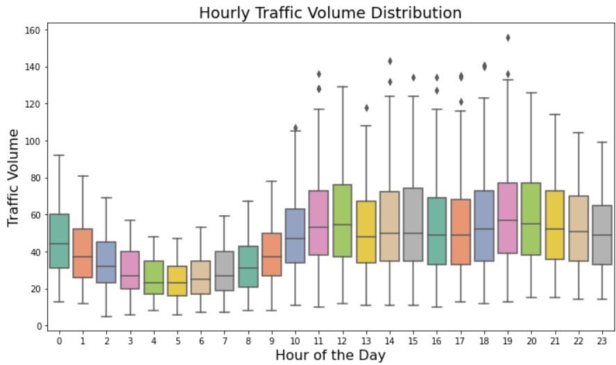
Hourly Traffic Volume Distribution: The box plot displays the distribution of traffic volume by hour of the day. Each box representing the range of traffic volumes observed in a particular hour. By examining the spread and median of each box, we can identify peak traffic hours with higher volumes and off-peak hours with lower volumes. This visualization aids in understanding the daily traffic patterns, highlighting the times when traffic congestion is most likely to occur.
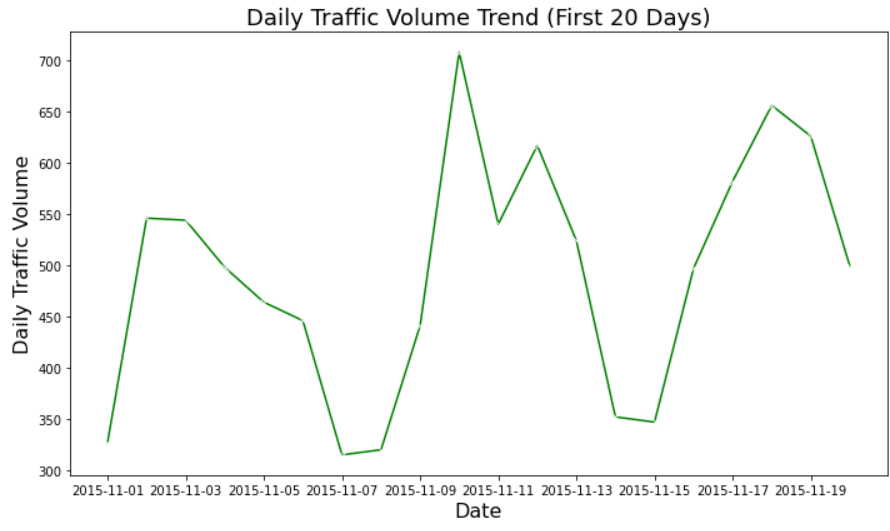
Daily Traffic Volume Trend: This line plot below presents the cumulative daily traffic volume at a specific junction. It showcases the total number of vehicles passing through over a 20-day period. Each point on the line represents the total traffic volume for that day. It allows us to observe patterns such as fluctuations in traffic flow. This visualization effectively illustrates the day-to-day variations in traffic volume, providing insights into peak traffic days and potential factors influencing these changes.
Visualizations clarify complex information and support informed decision-making. Building on these insights, we now turn our attention to the process of feature engineering. Feature engineering is where we refine and transform data to further enhance model performance.
Feature Engineering

In the realm of data analytics for traffic forecasting, a crucial preliminary step before training ML models is feature engineering. This process entails transforming the raw dataset into a format that’s more amenable to analysis by machine learning algorithms. It enhances their capability to deliver more accurate predictions for various aspects such as vehicle count, traffic flow, congestion levels, and travel times through advanced forecasting techniques. Good feature engineering is a foundation for learning algorithms. After all it transforms raw data into informative features that simplify the forecasting task and yield better results [9].
In feature engineering for datasets like traffic dataset, several key actions are considered, even if not implemented in given dataset. These actions can include the extraction of relevant attributes from the data, handling of missing values to ensure the integrity of the dataset, and encoding of categorical variables and normalization or scaling of numerical variables. These tasks help in preparing the data for machine learning models. Although the current dataset may not have undergone these specific transformations, they are standard practices in the process of making raw data more suitable for generating accurate machine learning predictions.
Furthermore, feature engineering may involve creating new features through methods like combining related attributes or decomposing existing ones into more granular components, as well as identifying the most impactful features that drive the accuracy of the model’s predictions. By refining and curating the dataset with these techniques, we can enhance the model’s ability to discern patterns and improve the precision of various traffic forecasting outcomes such as optimizing traffic flow, managing congestion, and improving travel time estimates. Additionally, selecting the most relevant features can reduce model complexity and enhance performance. Now let’s delve into some key elements of feature engineering for traffic forecasting:
- Data Extraction and Refinement: The initial step in feature engineering for the traffic dataset involves isolating key attributes that are crucial for traffic forecasting. This includes extracting the vehicle count, which serves as a direct measure of traffic volume, and the time of day, which is essential for capturing daily traffic patterns. Additionally, it’s important to ensure the dataset’s robustness by addressing any missing records. Incomplete data can lead to inaccurate predictions.
- Feature Transformation: Encoding categorical variables like junction IDs into a numerical format interpretable by machine learning models and normalizing numerical variables like vehicle count and time of day to prevent any single feature from disproportionately influencing the prediction due to its scale.
- Feature Creation and Selection: Generating new features by aggregating similar data points or decomposing complex traffic attributes into simpler ones, and choosing the most relevant features that enhance the predictive precision of the forecasting model. One valuable feature creation for the time of day is extracting specific time components, such as hour or part of the day (morning, afternoon, evening), which can provide more granular insights into traffic patterns and help improve the accuracy of the forecasting model.
- Optimization for Predictive Accuracy: The overarching goal is to refine the dataset, augmenting the model’s proficiency in recognizing patterns and determinants that affect traffic forecasting, thereby enhancing the reliability and utility of its predictions.
After having explored feature engineering, the next crucial stage is Model Training. This phase involves using the processed dataset, now optimized with carefully engineered features, to train the machine learning model on discerning the intricacies of various factors influencing traffic flow and congestion. With this foundational work in place, we are now ready to advance to the topic of training the model.
Training the Model
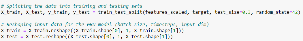
After preparing the dataset through feature engineering, the next stage is Model Training. In this phase, the machine “learns” to discern between various factors influencing traffic patterns, such as vehicle count, time of day, junction IDs, and potentially weather conditions. The dataset is divided into training and testing groups, a crucial step to ensure the model is trained on a specific subset of data while its performance is evaluated on another set of unseen data.
As emphasized earlier, this article does not aim to serve as an exhaustive tutorial on machine learning. Rather, its purpose is to showcase how machine learning techniques can be applied to analyze and optimize various aspects of traffic prediction.
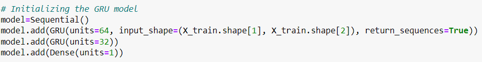
The following code snippets are designed to lay the groundwork for the various steps involved in training a model for traffic prediction. While the details may not constitute a complete program, they provide a glimpse into the type of approach required to build and train a model tailored for analyzing traffic patterns.


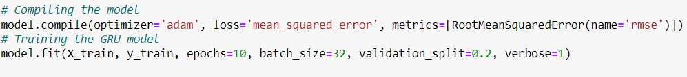
Moving forward, we’ll explore the Model Interpretation phase. We will focuse on how our model predicts various aspects of traffic flow and congestion. Here, the emphasis isn’t on the complexity of the model but on its accuracy and reliability. It’s crucial to understand that the model does more than just churn out predictions. It provides insights into traffic patterns and trends, translating raw data into actionable intelligence. In simpler terms, the goal is not only to assess if the model is effective but also to understand the mechanics behind its predictions and the reasons we can trust its guidance. This comprehension is key to confidently relying on the model for strategic decision-making processes in optimizing traffic management and planning.
Model Interpretation

In the context of traffic prediction using machine learning, model interpretation is centered around understanding how algorithms analyze traffic data. This data includes vehicle counts, time of day, and junction IDs to optimize traffic flow and management. This phase is crucial for ensuring that the insights provided by the model are not only accurate but also meaningful, explainable, and actionable. Explainability is valuable even when it’s not explicitly demanded by regulators or customers. After all, it fosters a level of transparency that builds trust with stakeholders. Emphasizing explainability is a critical component of ethical machine learning practices. It aims to underscore its importance in the development and deployment of predictive models for traffic management.
Interpreting these “black box” models can be challenging, as it requires simplifying complex algorithms without losing essential details. It extends beyond mere prediction accuracy. In fact, it involves unraveling the factors that influence traffic patterns and identifying trends that might not be immediately apparent. For example, understanding how a change in time of day or junction configuration impacts traffic flow can offer valuable insights for improving traffic management and optimizing resource allocation.
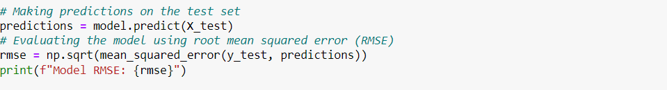
Evaluating model performance involves analyzing key metrics to assess the effectiveness of the traffic prediction system. Model evaluation plays a pivotal role in this process. It offers a quantitative measure of the model’s predictive capabilities in the context of traffic management.
- Mean Absolute Error (MAE): Measures the average magnitude of the errors in a set of predictions. It provides an indication of how close the forecasts are to the actual observations in terms of traffic volume.
- Root Mean Squared Error (RMSE): Measures the square root of the average of the squared differences between predicted and actual values, giving a higher weight to larger errors in traffic predictions.
Situational Metrics:
- Congestion Metrics: These metrics evaluate the impact of the model’s recommendations on traffic congestion levels, such as average speed, queue length, and delay time. They assess the practical value of the model in reducing congestion and improving traffic flow.
- Time-based Metrics: These metrics assess the operational efficiency of the model, including its runtime and the frequency of retraining required. They are particularly important in traffic management, where timely decision-making is critical.
These metrics, alongside advanced interpretability and explainability techniques such as feature importance rankings and partial dependence plots. These aid in demystifying the model’s decision-making process. They allow traffic planners & operators to refine traffic management strategies, optimize prediction accuracy. Also enhancing the understanding of complex traffic systems.
Key Takeaways
This article explores the pivotal role of machine learning in advancing traffic prediction, shedding light on its impact on urban commuting and transportation systems. By delving into the analysis of traffic data, it underscores how machine learning algorithms are employed to enhance the accuracy of traffic flow forecasts. The discussion encompasses feature engineering, model training, and interpretation, providing a comprehensive overview of the technical methodologies that underlie improved predictive performance. Through illustrative code examples, the article demonstrates the practical application of these techniques in optimizing traffic management and route planning. Ultimately, the article highlights the significant influence of machine learning in revolutionizing traffic prediction. It aims to encourage readers to explore the intersection of data science and transportation, with a focus on traffic forecasting advancements.
Next Steps
- Technology-related roles are the fastest growing jobs in percentage terms, including Big Data Specialists, AI and Machine Learning Specialists and Software and Application Developers [10]. This insight from the World Economic Forum’s Future of Job’s 2025 report highlights the growing demand in these fields.[10]. To position yourself advantageously in the job market, consider WeCloudData’s bootcamps. If you are interested in becoming a machine learning engineer, do check Weclouddata’s AI and Machine Learning bootcamp. Earn your Machine learning Certificate to start your Machine Learning Engineer Specialist Journey today! With real client projects, one-on-one mentorship, and hands-on experience in our immersive programs, it’s an opportunity to develop expertise in AI and machine learning. Align your skills with the current and future needs of the job market. Set yourself up for success in a dynamic and rewarding career; take action now!
References
[1] Yin, X., Wu, G., Wei, J., Shen, Y., Qi, H., & Yin, B. (2020). Deep Learning on Traffic Prediction: Methods, Analysis and Future Directions. arXiv preprint arXiv:2004.08555. Retrieved from https://ar5iv.labs.arxiv.org/html/2004.08555
[2] Abduljabbar, R. & Dia, H. Predictive Intelligence: a neural network learning system for traffic condition prediction and monitoring on freeways. J. Eastern Asia Soc. Transp. Stud. 13, 1785–1800 (2019). Retrieved from https://www.nature.com/articles/s41598-021-03282-z#ref-CR1
[3] Abduljabbar, R., Dia, H., Liyanage, S. & Bagloee, S. A. Applications of artificial intelligence in transport: an overview. Sustainability 11(1), 189 (2019). Retrieved from https://www.nature.com/articles/s41598-021-03282-z#ref-CR1
[4] Mahamuni, A. Internet of Things, machine learning, and artificial intelligence in the modern supply chain and transportation. Defense Transp. J. 74, 14–17 (2018). Retrieved from https://www.nature.com/articles/s41598-021-03282-z#ref-CR1
[5] Ma, X., Tao, Z., Wang, Y., Yu, H. & Wang, Y. Long short-term memory neural network for traffic speed prediction using remote microwave sensor data. Transp. Res. Part C Emerging Technol. 54, 187–197 (2015). Retrieved from https://www.nature.com/articles/s41598-021-03282-z#ref-CR1
[6] Kang, D., Lv, Y. & Chen, Y. Y. Short-term traffic flow prediction with LSTM recurrent neural network. In 2017 IEEE 20th International Conference on Intelligent Transportation Systems (ITSC) 1–6 (IEEE, 2017). Retrieved from https://www.nature.com/articles/s41598-021-03282-z#ref-CR1
[7] Zhao, Z., Chen, W., Wu, X., Chen, P. C. & Liu, J. LSTM network: a deep learning approach for short-term traffic forecast. IET Intel. Transport Syst. 11(2), 68–75 (2017). Retrieved from https://www.nature.com/articles/s41598-021-03282-z#ref-CR1
[8] Lau, J. (2020). Google Maps 101: How AI helps predict traffic and determine routes. Google Blog. Retrieved from https://blog.google/products/maps/google-maps-101-how-ai-helps-predict-traffic-and-determine-routes/
[9] Rawat, T., & Khemchandani, V. (2019). Feature Engineering (FE) Tools and Techniques for Better Classification Performance. International Journal of Innovations in Engineering and Technology, 8(2). DOI: 10.21172/ijiet.82.024.
[10 ] World Economic Forum (2025). “Future of Jobs Report 2025.” Retrieved from https://reports.weforum.org/docs/WEF_Future_of_Jobs_Report_2025.pdf.
